Introduction
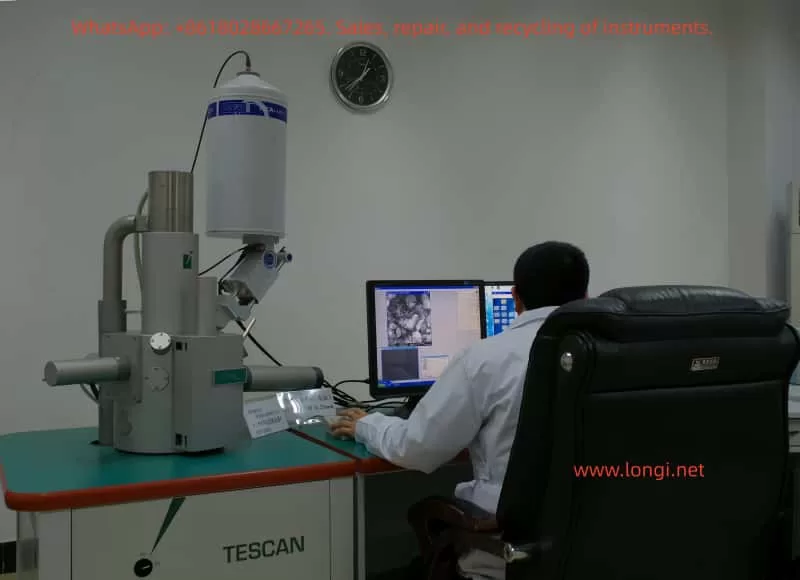
The Oxford INCA Energy Spectrometer is a high-end analytical instrument that integrates X-ray Energy Dispersive Spectroscopy (EDS) and electron microscope imaging capabilities. It is widely used in various fields such as materials science, geology, and biology. This guide aims to provide users with a comprehensive and systematic user guide by interpreting the Oxford INCA Energy Spectrometer’s operation manual, helping users quickly master the instrument’s operational techniques and improve analytical efficiency and accuracy.
I. System Overview and Component Introduction

1.1 System Composition
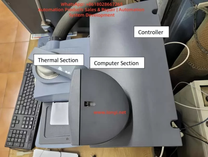
The Oxford INCA Energy Spectrometer system primarily consists of the following components:
- PC Host: Equipped with INCA Energy software for data processing and analysis.
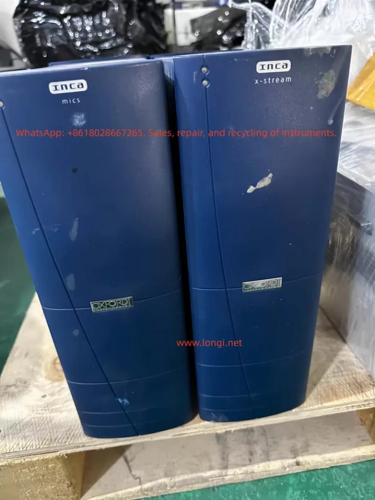
- x-stream Module: Controls X-ray acquisition.
- mics Module: Controls imaging functions.
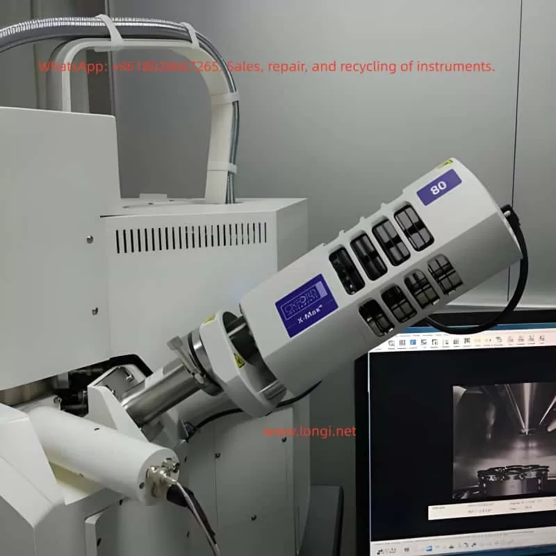
- EDS Detector: Detects X-rays and converts them into electrical signals.
- IEEE 1394 Card: Facilitates high-speed data transfer between the PC and hardware modules.
1.2 Software Interface Overview
The INCA Energy software platform comprises four main components:
- Navigators: Guide users through various stages of the microanalysis process, from initiating a new project to generating hardcopy reports.
- Data Management: Archives data in a logical and easily accessible manner, supporting viewing and management via a data tree.
- Help: Provides an online multimedia user help system, including bubble help, tooltips, and a microanalysis encyclopedia.
- Energy Options: Offers basic and advanced software option configurations to meet different user needs.
II. Project and Data Management
2.1 Project Creation and Management
In the INCA Energy software, all data is managed in the form of projects. Each project contains one or more samples, and each sample can include multiple sites of interest. Users can create and manage projects through the following steps:
- Create a New Project: Initiate a new project via the menu bar’s “File” -> “New Project” and specify the project’s save path and name.
- Add Samples: Right-click on “Samples” in the project data tree and select “Add Sample” to add a new sample.
- Define Sites of Interest: Right-click on “Sites of Interest” under a sample and select “Add Site” to define a new analysis area.
2.2 Data Management
The INCA Energy software offers robust data management capabilities, allowing users to view and manage all data intuitively through the data tree. Each entry in the data tree represents a specific data object, such as electron images, spectra, or elemental maps. Users can perform various operations, such as renaming, deleting, and exporting, by right-clicking on data entries.
2.3 Data Export and Sharing
The INCA Energy software supports exporting data in various formats for compatibility with other software packages. Users can export data through the following steps:
- Export Spectra: Right-click on a spectrum entry in the data tree, select “Export,” and then choose the desired file format (e.g., BMP, TIF, JPG, EMSA).
- Export Images and Maps: Similarly, users can right-click on image or map entries and select “Export” to export them in appropriate file formats.
- Copy Data to Clipboard: Users can also right-click on data entries and select “Copy” to copy data to the clipboard, then paste it into other applications.
III. Microscope Condition Optimization
3.1 Sample Tilt Correction
If the sample is tilted and requires quantitative analysis, users need to input the correct sample tilt value. If equipped with microscope control software and a motorized sample stage, the current tilt angle will be automatically read by the software. Otherwise, users must manually input the tilt value.
3.2 Accelerating Voltage Setting
The choice of accelerating voltage significantly impacts X-ray excitation and signal quality. Users should select an appropriate accelerating voltage based on sample characteristics and analysis requirements. A general recommendation is to start with 20kV, especially for unknown samples, as this voltage can excite X-rays from most elements.
3.3 Beam Current Setting
Beam current settings directly affect X-ray count rates and signal intensity. Users should adjust the beam current based on sample characteristics and analysis requirements to obtain sufficient count rates and a good signal-to-noise ratio. When setting the beam current, users should observe the filament saturation point to ensure beam stability.
3.4 Working Distance Adjustment
The working distance is defined as the distance between the objective lens’s lower pole piece and the electron beam’s focal plane. Users should adjust the working distance based on the EDS detector’s installation geometry in the SEM chamber to achieve optimal X-ray detection efficiency.
IV. X-ray Acquisition and Optimization
4.1 Quantitative Optimization (Quant Optimization)
Quantitative optimization is crucial for ensuring the accuracy of X-ray spectra. By performing quantitative optimization, the software can measure and store key parameters such as system gain and spectrometer resolution, thereby improving the accuracy of subsequent quantitative analyses. Users should perform quantitative optimization at the beginning of each new session or when system conditions change.
4.2 Optimal Acquisition Condition Selection
Users should select appropriate acquisition conditions based on analysis requirements, including livetime, process time, and spectrum energy range.
- Livetime: Specifies the duration for which the system processes X-ray signals.
- Process Time: Affects noise filtering and peak resolution settings. Longer process times reduce noise but slow down acquisition speed.
- Spectrum Energy Range: Selected based on accelerating voltage and analysis requirements.
4.3 Spectrum Acquisition and Display
Users can control spectrum acquisition using function keys (e.g., F9 to start, F10 to stop, F11 to resume). Acquired spectra can be displayed and manipulated in various ways within the software, including full-screen display, solid line display, and smart peak labeling.
V. Quantitative Analysis and Result Interpretation
5.1 Quantitative Analysis Workflow
Quantitative analysis involves several key steps:
- Background Subtraction: Suppresses background signals using digital filtering techniques.
- Peak Fitting: Uses standard peak shapes to perform least-squares fitting on the spectrum to extract peak areas for each element.
- Matrix Correction: Applies the XPP matrix correction scheme to correct measurement results, accounting for X-ray absorption and fluorescence effects.
- Result Output: Displays quantitative analysis results, including weight percentages for each element and the fit index.
5.2 Result Interpretation and Validation
Users should interpret sample composition based on quantitative analysis results and validate the accuracy of these results by comparing them with standard samples or samples of known composition. If the analysis results do not match expectations, users should verify that acquisition conditions, quantitative optimization, and matrix corrections were correctly executed.
VI. Advanced Features and Applications
6.1 SmartMap Functionality
The SmartMap feature allows users to simultaneously acquire X-ray data for all possible elements from each pixel in an image. This analysis method offers high flexibility and is suitable for various complex samples. Users can optimize analysis results by setting SmartMap resolution, process time, and acquisition time parameters.
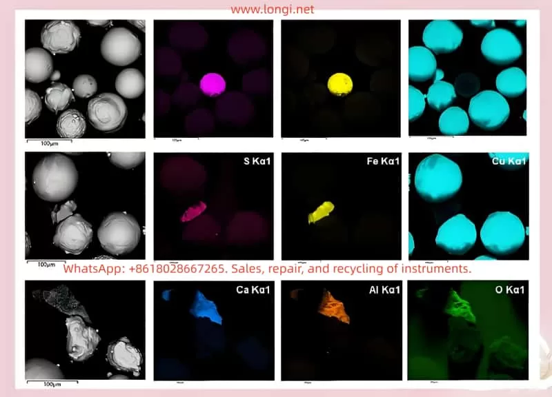
6.2 Elemental Mapping and Line Scanning
Elemental mapping and line scanning features enable users to visualize the distribution of elements within a sample. Users can generate elemental maps or line scan images by selecting specific X-ray lines and adjust display parameters to achieve optimal visualization.
6.3 Cameo+ Functionality
The Cameo+ feature combines electron images with X-ray spectral information to display the chemical composition and topography of a sample in a color overlay. Users can adjust the color range to highlight specific compositional variations within the sample.
6.4 PhaseMap Functionality
The PhaseMap feature displays the distribution of different phases within a sample using scatter plots. Users can use Cameo+ data or elemental map data as the source for PhaseMap and identify different phases within the sample through cluster analysis.
6.5 AutoMate Functionality
The AutoMate feature allows users to set up a series of automated tasks, such as repeatedly acquiring spectra or images at different locations. This is particularly useful for applications requiring uniform analysis over large areas or long-term monitoring.
VII. Maintenance and Troubleshooting
7.1 Routine Maintenance
Users should perform routine maintenance on the INCA Energy Spectrometer, including cleaning the sample chamber, checking detector status, and calibrating the microscope. Additionally, users should regularly back up project data to prevent data loss.
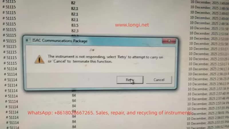
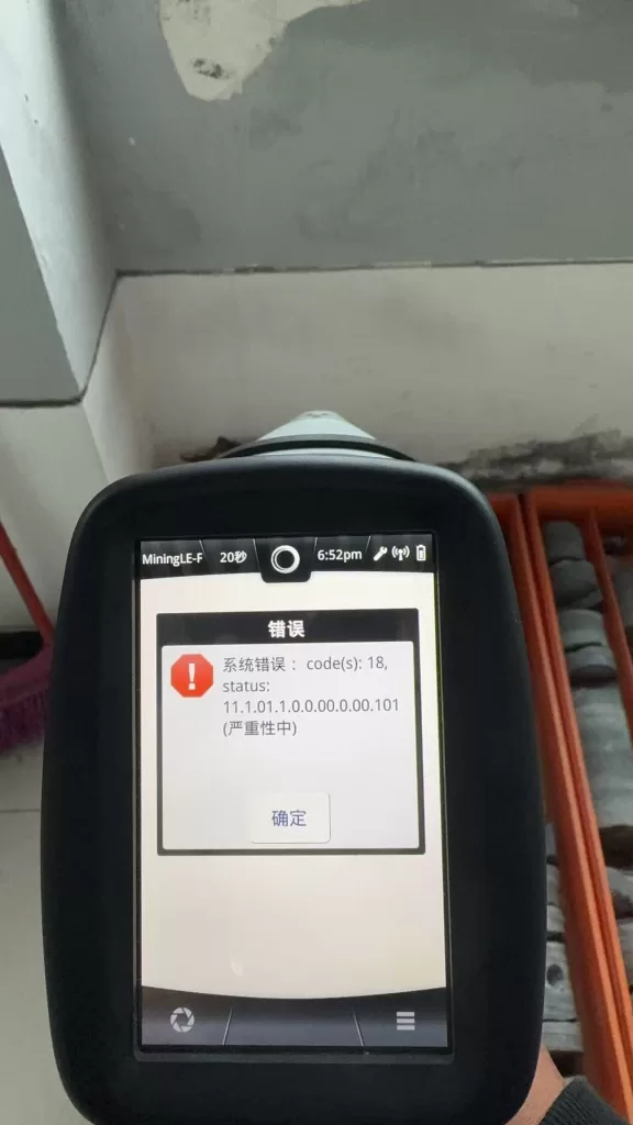
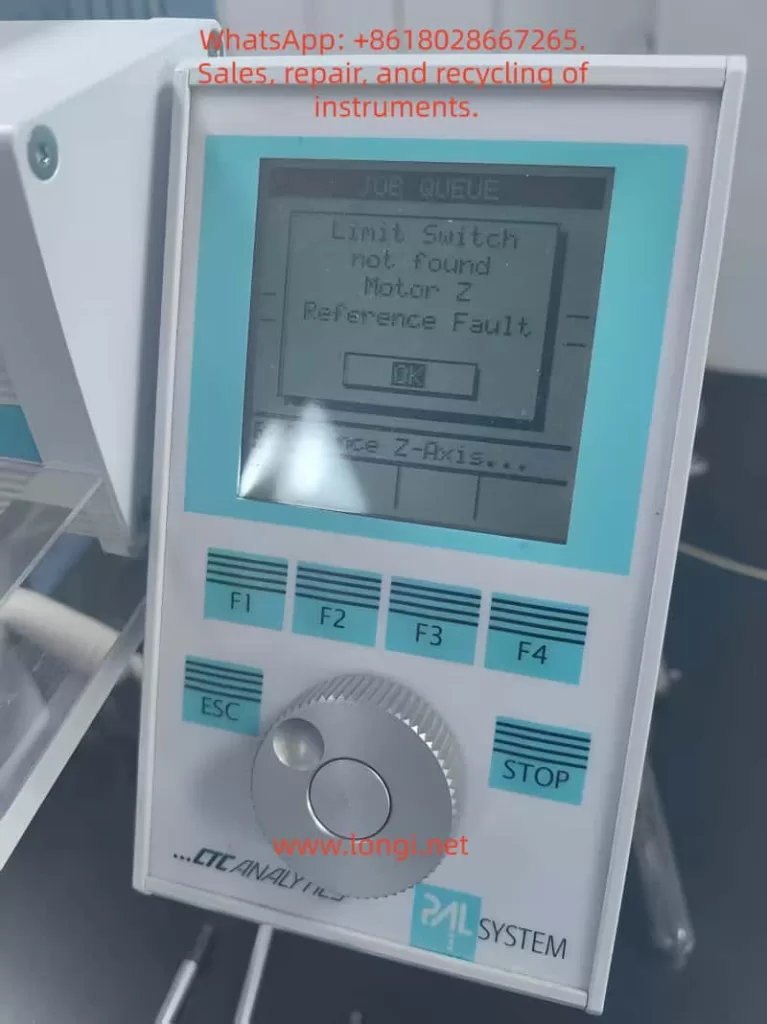
7.2 Troubleshooting
If problems arise during use, users can refer to the troubleshooting section of the operation manual or contact Oxford Instruments’ technical support team for assistance. Common issues include detector saturation, weak signals, and software crashes. Users should take appropriate corrective measures based on the specific situation.
Conclusion
This guide provides a comprehensive and systematic user guide by interpreting the Oxford INCA Energy Spectrometer’s operation manual. By mastering the operational techniques and methods introduced in this guide, users can more efficiently and accurately use the INCA Energy Spectrometer for various analytical tasks. We hope this guide proves helpful to a wide range of users and promotes the application and development of the INCA Energy Spectrometer in various fields.